3.1. Introduction
The most convenient geometrical arrangement for the field analysis of a loop antenna is to position the antenna symmetrically on the \(x-y\) plane, at \(z = 0\). The wire is assumed to be very thin and the current is assumed to be constant. A constant current distribution is accurate only for a loop antenna with a very small circumference [8].

Fig. 3.1 : Geometrical arrangement for loop antenna analysis
In the analysis of radiation problems, the usual procedure is to specify the sources and then require the fields radiated by the sources. It is a very common practice in the analysis procedure to introduce auxiliary functions, known as vector potentials, which will aid in the solution of the problems. The most common vector potential functions are the \(A\) (magnetic vector potential) and \(F\) (electric vector potential). While it is possible to determine the \(E\) and \(H\) fields directly from the source-current densities \(J\) and \(M\), as shown in Fig. 3.1, it is usually much simpler to find the auxiliary potential functions first and then determine the \(E\) and \(H\). This two-step procedure is also shown in Fig. 3.1 [8].
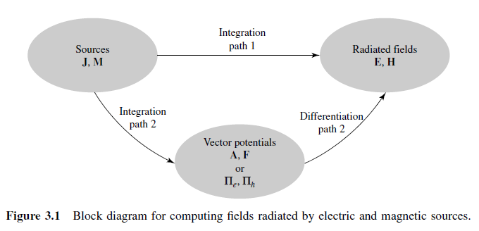
Fig. 3.2 : Block diagram for computing fields radiated by electric and magnetic sources.
Defining properties for an electrically small antenna are low directivity, low input resistance, high input reactance and low radiation efficiency [Stutzman and Thiele, 2012].
# In practice, a dipole antenna is usually operated at or near its first resonant frequency. However, electrically small antennas, such as active receiving antennas, operate well below the resonant frequency [58].